A Basic Introduction to Algorithms using JavaScript

My notes taken from "Complete Intro to Computer Science" by Brian Holt in Frontend Masters course.

• Big O Time Complexity
• Spatial Complexity
• Iterative Sorts
• Bubble Sort
• Insertion Sort
• Recursive Sorts
• Merge Sort
• Quick Sort
• Non-Comparison Sorts
• Radix Sort
• Binary Search
• References

Big O Time Complexity

What is Big O

It’s a method used to measure how efficient is an algorithm without getting into too much details, if you don’t know how it works you can’t judge if your algorithm is getting faster or slower.

Think of the O as a vacuum that sucks in all the unimportant information and just leaves you with the important stuff.

Say we have the equation $3x^2 + x + 1$. If our input is 5, the first term will be 75, the second term will be 5, and the third will be 1.

A “term” in mathematics just means one piece of the equation (normally separated by + or - signs). In $3x^2 + x + 1$, $3x²$ is the first term, $x$ is the second, and $1$ is the third.

In other words, most of the piece of the pie comes from the first term, to the point we can just ignore the other terms. If we plug in huge numbers, it becomes even more apparent. IE if we do 5,000,000, the first term is 75,000,000,000,000, the second is 5,000,000, and the last 1. A huge gap.

We ignore the little parts and concentrate on the big parts. Keeping with $3x² + x + 1$, the Big O for this equation would be O(n²) where O is just absorbing all the other fluff (including the factor on the biggest term.) Just grab the biggest term.

In industry (and therefore in interviews), people seem to have merged Big $\theta$ (Theta) and Big O together. Industry’s meaning of Big O is closer to what academics mean by $\theta$.

Time Complexity Classes

The time of the algorithm is greatly affected depending on the input. Here we can see a graphical example.

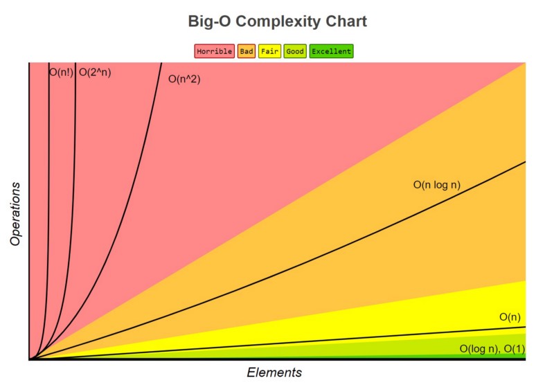
Constant O(1)

The number of operations stays the same, independent of the number of elements.

Logarithmic O(log n)

The number of operations increases by a constant amount whenever the number of elements doubles.

Linear O(n)

The number of operations grows linearly with the number of elements n. If n doubles, the number of operations doubles, too

Quasilinear O(n log n)

The number of operations grows slightly faster than linear as the linear component is multiplied with a logarithmic one.

Exponential O(2$^n$)

The number of operations grows linearly with the square of the number of elements n. If n doubles, the number of operations quadruples

Factorial O(n!)

The number of operations grows linearly with the factorial of the number of elements n, which is the product of all numbers up to (and including) n.

Big O Example 1

function findNumber(nums, value){
  for(let i = 0; i < nums.length; i++) {
    if(nums[i] == value) return true;
  }

  return false;
}

This code is $n + 1$ because it has a loop that depends on the quantity of entries on input and also has some commands that doesn’t not depend of input.

Ignore the $+ 1$ because it’s not relevant close to $n$, now we are left with O(n), which is the Big O of this algorithm.

Big O Example 2

function combineAndPrintNums(nums){
  let combinedNums = [];

  for(let i = 0; i < nums.length; i++){
    for(let j = 0; j < nums.length; j++){
      combinedNums.push(nums[i] + nums[j]);
    }
  }

  for(let i = 0; i < combinedNums.length; i++){
    console.log(combindNums[i]);
  }
}

Now, this code is $n^2 + n + 1$, we just ignore the smaller terms… The big O is O($n^2$)

Spatial Complexity

What is Spatial Complexity

Spatial Complexity is the amount of space (e.g. how much RAM or disk space) an algorithm needs to complete.

Spatial Complexity Classes

One space complexity algorithm isn’t necessarily better than the other. And very frequently you need to make the trade off of computational complexity vs spatial. Some algorithms eat a lot of memory but go fast and there are lots that eat zero memory but go slow. It just depends on what your needs are.

Linear

Let’s say we have an algorithm that for every item in the array, it needs to create another array in the process of sorting it. So for an array of length 10, our algorithm will create 10 arrays. For an array of 100, it’d create 100 extra arrays. This would be O(n) in terms of its spatial complexity.

Logarithmic

What about another for every item in the array, it needed to create a diminishing amount of extra arrays. For example: for an array of length 10, it’d create 7 arrays. For an array of 100, it’d create 12 arrays. For an array of 1000, it’d created 20 arrays. This would be O(log n).

Constant

What if we didn’t create any extra arrays when we did our algorithm? We just used the same space we were given when we first started. Or if we created just 10 arrays, no matter how long the array is? This would be O(1) since it’s constant no matter what. Its spatial need don’t increase with longer arrays.

Quadratic

Let’s say we input a array into our algorithm that contains 10 elements. If we create exact 10 (length of the input array) extra arrays for each element, than that would be an example of a quadratic spatial time complexity, O(n$^2$).

Iterative Sorts

Bubble Sort

Normally Bubble Sort is not used in real life scenarios due to how it scales with larger amounts of data, but is a good teaching algorithm.

• The algorithms pops up the numbers to the top, just like a bubble (that’s a good way of reminding how it works).

• The algorithm loops through the list and swaps numbers if they are larger than the next.

• If you did not swap items, your list is sorted.

• If you swapped items, then you have to loop again and again, until no swaps happens.

Step-by-step example

[1, 5, 4, 2, 3]

Are 1 and 5 out of order? No.
Are 5 and 4 out of order? Yes. Swap.

[1, 4, 5, 2, 3]

Are 5 and 2 out of order? Yes. Swap.

[1, 4, 2, 5, 3]

Are 5 and 3 out of order? Yes. Swap.

[1, 4, 2, 3, 5]

End of the array, did we swap anything? Yes. Loop again.
Are 1 and 4 out of order? No.
Are 4 and 2 out of order? Yes. Swap.

[1, 2, 4, 3, 5]

Are 4 and 3 out of order? Yes. Swap.

[1, 2, 3, 4, 5]

Are 4 and 5 out of order? No.
End of the array, did we swap anything? Yes. Loop again.
Are 1 and 2 out of order? No.
Are 2 and 3 out of order? No.
Are 3 and 4 out of order? No.
Are 4 and 5 out of order? No.
End of the array, did we swap anything? No. List is sorted.

JavaScript Code Example

function BubbleSort(nums){
  let notSwapped = true;

  while(notSwapped){
    let swaps = 0;

    for(let i = 0; i < nums.length - 1; i++){
      if(nums[i] > nums[i + 1]){
        let aux;
        aux = nums[i];
        nums[i] = nums[i + 1];
        nums[i + 1] = aux;
        swaps++;
      }
    }

    if(swaps == 0){
      notSwapped = false;
    }
  }

  return nums;
}

Best, worst, and average cases

The best case scenario of this sorting algorithm should be a sorted list, since all the numbers are already sorted, no swaps happen, so one iteration is enough, O(n).

The worst case scenario of this is a reversed sorted list, since you have to iterate for every swap, O(n$^2$)

Average case looks like O(log n) since we are making less swaps then the length of the input, but if you have a larger set of data, it’s not gonna be any different than O(n$^2$).

Spatial Complexity

We don’t create any extra array using this algorithm, so that would be constant O(1).

Insertion Sort

This algorithm stars at index 1 (assuming we are starting at 0), compares the index with the left part of the array and inserts it in the right place.

• Insertion sort is one of the fastest algorithms for sorting very small arrays, even faster than quicksort.

Step-by-step example

[3, 2, 5, 4, 1]

    ↓
[3, 2, 5, 4, 1] // the ↓ is the number we're looking to insert, everything before is sorted

Is 2 larger than 3? No. Move 3 to the right.
Beginning of list, insert 2 at index 0.

       ↓
[2, 3, 5, 4, 1]

Is 5 larger than 3? Yes.
Insert after 3 (it's already there so it doesn't move)

          ↓
[2, 3, 5, 4, 1]

Is 4 larger than 5? No. Move 5 to the right.
Is 4 larger than 3? Yes.
Insert after 3 at index 2.

             ↓
[2, 3, 4, 5, 1]

Is 1 larger than 5? No. Move 5 to the right.
Is 1 larger than 4? No. Move 4 to the right.
Is 1 larger than 3? No. Move 3 to the right.
Is 1 larger than 2? No. Move 2 to the right.
Beginning of list, insert 1 at index 0

[1, 2, 3, 4, 5]

Reached end of list, list is sorted.

JavaScript Code Example

function insertionSort(nums) {
  for (let i = 1; i < nums.length; i++) {
    let numberToInsert = nums[i];
    let j;

    for (j = i - 1; nums[j] > numberToInsert && j >= 0; j--) {
      nums[j + 1] = nums[j];
    }

    nums[j + 1] = numberToInsert;
  }
  return nums;
}

Best, worst, and average cases

The best case input is an array that is already sorted. In this case insertion sort has a linear running time O(n).

The simplest worst case input is an array sorted in reverse order, resulting in O(n$^2$).

The average case is also quadratic O(n$^2$), which makes insertion sort impractical for sorting large arrays. However, insertion sort is one of the fastest algorithms for sorting very small arrays, even faster than quicksort.

Spatial Complexity

Insertion Sort does not create any extra array, so it’s constant time O(1).

Recursive Sorts

Merge Sort

Merge Sort is a divide-and-conquer algorithm. It works by dividing the input into equal parts until only two numbers are there for comparisons and then after comparing and ordering each parts it merges them all together back to the input.

Step-by-step example

mergeSort([1, 5, 7, 4, 2, 3, 6]) -- depth 0

mergeSort([1, 5, 7, 4]) // mergeSort([2, 3, 6]) -- depth 1

mergeSort([1, 5]) // mergeSort([7, 4]) -- depth 2

mergeSort([1]) // mergeSort([5]) -- depth 3
[1] is of length one. Base case. Return sorted list [1] -- depth 3

mergeSort([5]) -- depth 3
[5] is of length one. Base case. Return sorted list [5] -- depth 3

merge([1], [5]) -- depth 3
Is 1 or 5 smaller? 1. Add to end. [1]
Left array is empty, concat right array. [1, 5]
Return sorted array [1, 5].

mergeSort([7, 4]) -- depth 2

mergeSort([7]) // mergeSort([4]) -- depth 3
[7] is of length one. Base case. Return sorted list [7] -- depth 3

mergeSort([4]) -- depth 3
[4] is of length one. Base case. Return sorted list [4] -- depth 3

merge([7], [4]) -- depth 3
Is 7 or 4 smaller? 4. Add to end. [4]
Right array is empty, concat left array. [4, 7]
Return sorted array [4, 7]

merge([1, 5], [4, 7]) -- depth 2
Is 1 or 4 smaller? 1. Add to end. [1]
Is 5 or 4 smaller? 4. Add to end. [1, 4]
Is 5 or 7 smaller? 5. Add to end. [1, 4, 5]
Left array is empty, concat right array. [1, 4, 5, 7]
Return sorted array [1, 4, 5, 7]

mergeSort([2, 3, 6]) -- depth 1

mergeSort([2, 3]) // mergeSort([6]) -- depth 2

mergeSort([2]) // mergeSort([3]) -- depth 3
[2] is of length one. Base case. Return sorted list [2]

mergeSort([3]) -- depth 3
[3] is of length one. Base case. Return sorted list [3]

merge([2], [3]) -- depth 3
Is 2 or 4 smaller? 2. Add to end. [2]
Left array is empty, concat right array. [2, 3]
Return sorted array [2, 4]

mergeSort([6]) -- depth 2
[6] is of length one. Base case. Return sorted list [6]

merge([2, 3], [6]) -- depth 2
Is 2 or 6 smaller? 2. Add to end. [2]
Is 3 or 6 smaller? 3. Add to end. [2, 3]
Left array is empty, concat right array. [2, 3, 6]
Return sorted array [2, 3, 6]

merge([1, 4, 5, 7], [2, 3, 6]) -- depth 1
Is 1 or 2 smaller? 1. Add to end. [1]
Is 4 or 2 smaller? 2. Add to end. [1, 2]
Is 4 or 3 smaller? 3. Add to end. [1, 2, 3]
Is 4 or 6 smaller? 4. Add to end. [1, 2, 3, 4]
Is 5 or 6 smaller? 5. Add to end. [1, 2, 3, 4, 5]
Is 7 or 6 smaller? 6. Add to end. [1, 2, 3, 4, 5, 6]
Right array is empty, concat left array. [1, 2, 3, 4, 5, 6, 7]
Return sorted list [1, 2, 3, 4, 5, 6, 7]

JavaScript Code Example

function MergeSort(arr) {
  if(arr.length < 2) return arr;

  const middle = Math.floor(arr.length / 2);
  const left = arr.slice(0, middle);
  const right = arr.slice(middle);

  const sortedLeft = MergeSort(left);
  const sortedRight = MergeSort(right);

  return Merge(sortedLeft, sortedRight);
}

function Merge(left, right) {
  const results = [];

  while(left.length && right.length){
    if(left[0] <= right[0]){
      results.push(left.shift());
    } else {
      results.push(right.shift());
    }
  }

  return results.concat(left, right);
}

Best, worst, and average cases

With Merge Sort every case is the worst case scenario. And the best. And the average. No matter what, the array always gets broken down into lists of 1 and then built back up, which ends it up by being O(n log n).

Spatial Complexity

For every element in our input Merge Sort will create an array, so it has a spatial complexity of O(n).

Quick Sort

It’s another divide-and-conquer, recursive algorithm but it takes a slightly different approach. It works by selecting a ‘pivot’ element from the array partitioning the other elements into sub arrays (left and right), according to whether they are less than or greater than the pivot. Calls Quick Sort recursively for both sub arrays. After those two sorts come back, you concatenate the sorted left list, the pivot, and then the right list.

Step-by-step example

[4,9,3,5] list
-> 5 is made the pivot since it's the last in the array
-> divide list into two lists, [4,3] and [9]
-> call quicksort on those two lists

[4, 3]
-> 3 is pivot
-> call quicksort on [] and [4]
-> those both return as is as they are the base case of length 0 or 1
-> concat [], 3, and [4]
-> return [3,4]

[9]
-> returns as this it is a base case of length 1

(back into the original function call)
-> call concat on [3,4], 5, and [9]
-> return [3,4,5,9]

JavaScript Code Example

function QuickSort(arr){
  if(arr.length < 2) return arr;

  let pivot = arr[arr.length - 1];
  let left = [];
  let right = [];
  
  for(let i = 0; i < arr.length - 1; i++){
    if(arr[i] >= pivot) {
      right.push(arr[i]);
    } else {
      left.push(arr[i]);
    }
  }

  let sortedLeft = QuickSort(left);
  let sortedRight = QuickSort(right);

  return sortedLeft.concat(pivot, sortedRight);
}

Best, worst, and average cases

The best case would be a randomly sorted list, so the pivots are going to get a good mix on left and right arrays, so that would be O(n log n).

Worst cases would be a sorted list or reversed list since you always will create sub arrays for a individual side (right or left) comparing every number to every number, that would be O(n$^2$)

Average case should be the same as best case. O(n log n).

Spatial Complexity

Spatial complexity for quick sort is also O(n), same as merge sort. But there are some quick sort variations that make it better.

Non-Comparison Sorts

Radix Sort

Radix Sort is pretty easy to understand conceptually, but I found it pretty hard to implement this myself.

But uh, it’s a non-comparison sort. The way it works is by finding the longest, yes, longest not largest number in the array.

So.. In [9414, 1, 123, 145], 9414 is our longest number because it has 4 digits.

Then we need a data structure that has 10 arrays ranging from 0 to 9.

For each element in our input we have to insert into a bucket, the criteria is the last digit, if the last digit is 6 then insert into the 7th bucket 6.

Now we dequeue all the numbers the buckets to the array again, and now the criteria is the second digit, that goes on and on, then the list gets sorted.

Step-by-step example

-> [109, 224, 901, 58, 41]
Longest Digit Number -> 3

For the first digit insert into the right bucket: 

Buckets:  
0: [] 1: [901, 41] 2: [] 3: [] 4: [224] 

5: [] 6: [] 7: [] 8: [58] 9: [109]

Now dequeue all to the array again in order

-> [901, 41, 224, 58, 109]

For the second digit insert into the right bucket:
Buckets:  
0: [901] 1: [] 2: [] 3: [] 4: [41, 224] 

5: [] 6: [] 7: [] 8: [58] 9: [109]

Now dequeue all to the array again in order

-> [901, 41, 224, 58, 109]

For the third digit insert into the right bucket:
Buckets:  
0: [41, 58] 1: [109] 2: [224] 3: [] 4: [] 

5: [] 6: [] 7: [] 8: [] 9: [901]

Now dequeue all to the array again in order

Longest digit have been reached, list is sorted.

JavaScript Code Example

function getDigit(number, place, longestNumber) {
  const string = number.toString();
  const size = string.length;

  const mod = longestNumber - size;
  return string[place - mod] || 0;
}

function getLongestNumber(nums) {
  let longest = 0;

  for (let i = 0; i < nums.length; i++) {
    const currentLength = nums[i].toString().length;
    longest = currentLength > longest ? currentLength : longest;
  }

  return longest;
}

function RadixSort(nums) {
  const longestNumber = getLongestNumber(nums);

  const buckets = new Array(10).fill().map(() => [])

  for (let i = longestNumber - 1; i >= 0; i--) {
    while (nums.length) {
      const current = nums.shift();

      buckets[getDigit(current, i, longestNumber)].push(current);
    }

    for (let j = 0; j < 10; j++) {
      while (buckets[j].length) {
        nums.push(buckets[j].shift())
      }
    }
  }

  return nums;
}

Best, worst, and average cases

The Big O of this algorithm is always the same, because it will sort the same way, which is O($nw$), where $n$ is the number of keys, and $w$ the keys length.

Radix sort works pretty well with an input of numbers ranging from 100-1000.

Spatial Complexity

It’s not great considering how much it takes on space which is O(n + k).

Binary Search

Binary search is a better way of searching through a sorted array instead of a linear search.

The way binary search works is by looking for the element in the middle of the array, if you find, then return it.

If it’s larger then the middle then you look into the middle of the right part, if it’s not larger then you look into the middle of the left part.

So you just keep cutting half of the array until you find the element.

Step-by-step example

[0, 5, 10, 12, 15, 19, 21, 22, 24, 30]

search for 12

start in the middle, is 19 === 12? no, smaller, go left

look in the middle of the smaller half, 10 === 12? no, larger, go right

look in the middle of the larger half (which is now just one number), is 12 === 12? yes, found element

JavaScript Code Example

function BinarySearch(arr, id) {
  let min = 0;
  let max = arr.length - 1;
  let index;

  while (min <= max) {
    index = Math.floor((min + max) / 2);
    if (arr[index] == id) return arr[index];

    if (arr[index] < id) {
      min = index + 1;
    } else {
      max = index - 1;
    }
  }

  return false;
}

Best, worst, and average cases

Best case would be the element is in the middle that would require one iteration, so O(1).

Worst and average case is the same, this algorithm will keep halving the array until It cannot anymore.

Reference

• Complete Intro to Computer Science - Course Website
• Watch the course in Frontend Masters